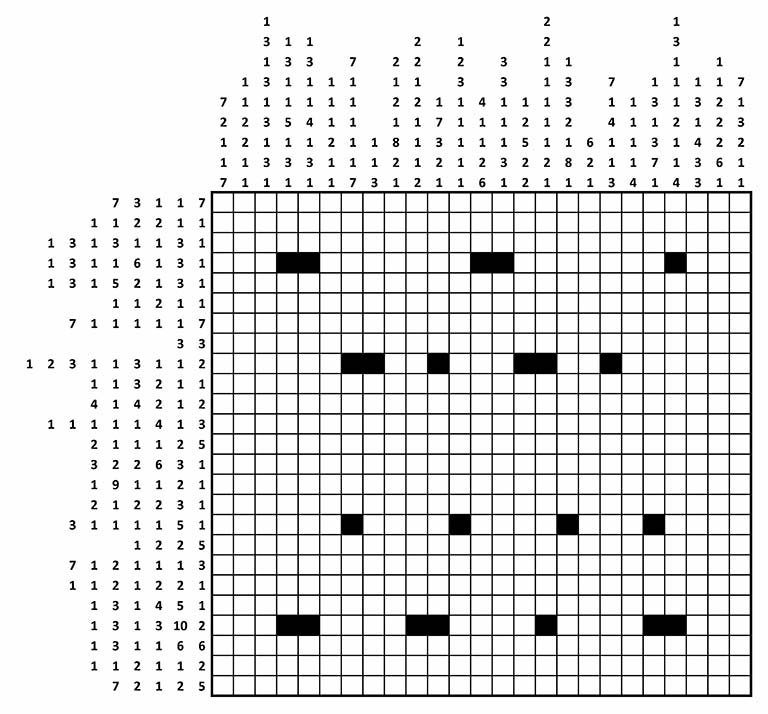
The GCHQ’s Christmas Challenge puzzle shown in the picture below has been making rounds on social media and in the news so I decided to try modeling it in AMPL and solving with a constraint programming solver.
Here are the rules of the puzzle:
In this type of grid-shading puzzle, each square is either black or white. Some of the black squares have already been filled in for you.
Each row or column is labelled with a string of numbers. The numbers indicate the length of all consecutive runs of black squares, and are displayed in the order that the runs appear in that line. For example, a label “2 1 6” indicates sets of two, one and six black squares, each of which will have at least one white square separating them.

The first step is declaring parameters and sets to represent the input data:
N: the number of rows or columns (they are the same in this problem)
param N > 0;
MaxRun: the maximum length of a run
param MaxRun > 0;
RC: a set of rows or columns to simplify indexing expressions.
set RC = 1..N;
RowRunLenandColRunLen: the lengths of row and column runs respectively with zero representing “no value” for the cases when the number of runs is smaller thanMaxRun
param RowRunLen{RC, 1..MaxRun} default 0;
param ColRunLen{RC, 1..MaxRun} default 0;
KnownPos: positions of known black squares
set KnownPos dimen 2;
RowRunsandColRuns: set of row and column runs respectively
set RowRuns = {r in RC, i in 1..MaxRun: RowRunLen[r, i] > 0};
set ColRuns = {c in RC, i in 1..MaxRun: ColRunLen[c, i] > 0};
The most challenging part of this particular puzzle for me was to enter the data. Fortunately AMPL has a powerful data specification language so I came up with a tabular format similar to the form used in the original puzzle which was easy to verify.
param ColRunLen (tr)
:  1  2  3  4  5  6  7  8  9 10 11 12 13 14 15 16 17 18 19 20 21 22 23 24 25 :=
1  .  .  1  .  .  .  .  .  .  .  .  .  .  .  .  2  .  .  .  .  .  1  .  .  .
2  .  .  3  1  1  .  .  .  .  2  .  1  .  .  .  2  .  .  .  .  .  3  .  .  .
3  .  .  1  3  3  .  7  .  2  2  .  2  .  3  .  1  1  .  .  .  .  1  .  1  .
4  .  1  3  1  1  1  1  .  1  1  .  3  .  3  .  1  3  .  7  .  1  1  1  1  7
5  7  1  1  1  1  1  1  .  2  2  1  1  4  1  1  1  3  .  1  1  3  1  3  2  1
6  2  2  3  5  4  1  1  .  1  1  7  1  1  1  2  1  2  .  4  1  1  2  1  2  3
7  1  2  1  1  1  2  1  1  8  1  3  1  1  1  5  1  1  6  1  1  3  1  4  2  2
8  1  1  3  3  3  1  1  1  2  1  2  1  2  3  2  2  8  2  1  1  7  1  3  6  1
9  7  1  1  1  1  1  7  3  1  2  1  1  6  1  2  1  1  1  3  4  1  4  3  1  1;

param RowRunLen
 :  1  2  3  4  5  6  7  8  9 :=
 1  .  .  .  .  7  3  1  1  7
 2  .  .  .  1  1  2  2  1  1
 3  .  1  3  1  3  1  1  3  1
 4  .  1  3  1  1  6  1  3  1
 5  .  1  3  1  5  2  1  3  1
 6  .  .  .  .  1  1  2  1  1
 7  .  .  7  1  1  1  1  1  7
 8  .  .  .  .  .  .  .  3  3
 9  1  2  3  1  1  3  1  1  2
10  .  .  .  1  1  3  2  1  1
11  .  .  .  4  1  4  2  1  2
12  .  1  1  1  1  1  4  1  3
13  .  .  .  2  1  1  1  2  5
14  .  .  .  3  2  2  6  3  1
15  .  .  .  1  9  1  1  2  1
16  .  .  .  2  1  2  2  3  1
17  .  .  3  1  1  1  1  5  1
18  .  .  .  .  .  1  2  2  5
19  .  .  7  1  2  1  1  1  3
20  .  .  1  1  2  1  2  2  1
21  .  .  .  1  3  1  4  5  1
22  .  .  .  1  3  1  3 10  2
23  .  .  .  1  3  1  1  6  6
24  .  .  .  1  1  2  1  1  2
25  .  .  .  .  7  2  1  2  5;

set KnownPos :=
 4  4
 4  5
 4 13
 4 14
 4 22
 9  7
 9  8
 9 11
 9 15
 9 16
 9 19
17  7
17 12
17 17
17 21
22  4
22  5
22 10
22 11
22 16
22 21
22 22;
Now to the interesting part: I used two sets of decision variables, RowRunStart and
ColRunStart, to represent start positions of row and column runs respectively:
var RowRunStart{(r, i) in RowRuns} integer >= 1 <= N;
var ColRunStart{(c, i) in ColRuns} integer >= 1 <= N;
A good thing about constraint programming formulation is that it is pretty straightforward because you can model logic, such as disjunctions, directly and don’t need to introduce binary variables as in MIP case.
This is a constraint satisfaction problem, so we don’t need an objective, just constraints. The first group of constraints makes sure that row runs don’t overlap and the same for column runs:
s.t. no_row_overlap{(r, i) in RowRuns: i < MaxRun}:
  RowRunStart[r, i] + RowRunLen[r, i] <= RowRunStart[r, i + 1] - 1;

s.t. no_col_overlap{(c, i) in ColRuns: i < MaxRun}:
  ColRunStart[c, i] + ColRunLen[c, i] <= ColRunStart[c, i + 1] - 1;
The next constraint links row and column runs by stating that every element of a row run should belong to some column run:
s.t. row_col_intersect{(r, i) in RowRuns, l in 0..RowRunLen[r, i] - 1}:
  exists{(c, j) in ColRuns} (c == RowRunStart[r, i] + l &&
                             ColRunStart[c, j] <= r &&
                             r < ColRunStart[c, j] + ColRunLen[c, j]);
It might be possible to model this more efficiently, but I didn’t bother because even this naive formulation was solved in less than a minute.
And the last constraint brings in known black squares stating that each of these squares should belong to some row run:
s.t. known_pos{(r, c) in KnownPos}:
  exists{(r, i) in RowRuns}
    RowRunStart[r, i] <= c && c < RowRunStart[r, i] + RowRunLen[r, i];
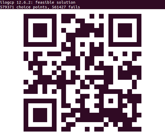
And that’s the whole formulation. The following little script solves it with
IBM ILOG CPLEX CP Optimizer
aka ilogcp and displays the solution in a terminal:
option solver ilogcp;
solve;

printf{1..35} '██';
print;
for {r in RC} {
  printf{1..5} '██';
  for {c in RC} {
    if exists{(r, i) in RowRuns} RowRunStart[r, i] <= c && c < RowRunStart[r, i] + RowRunLen[r, i] then
      printf '  ';
    else
      printf '██';
  }
  printf{1..5} '██';
  print;
}
printf{1..35} '██';
This worked pretty well and scanned with Barcode Scanner app on my phone although a fancier way would be to use something like iampl or AMPL API to render a proper image instead of using ASCII “art”.

And this post would be incomplete without mentioning related approaches to solving this puzzle, Solving The GCHQ Christmas Puzzle As A MIP With Python by Jean-Francois Puget and Solving the GCHQ christmas card with Python and pycosat by Matthew Earl.
You can find the complete AMPL code to solve this puzzle here.
Last modified on 2015-12-13