In this post I will give an introduction to iampl, a project which implements AMPL magics for IPython. IPython is a Python-based interactive environment with additional capabilities for visualization, rendering formulas, scientific computing, data introspection, etc. With iampl it is possible to use IPython as an interface to AMPL and do modeling, data processing and visualization in one rich environment. This post itself is also written using IPython.

You can download the latest version of iampl from here. The archive contains a Python module called ampl.py implementing the magics and a sample IPython notebook called example.ipynb. ~~To install iampl, place ampl.py in the directory~~

~~~/.config/ipython/profile_default/startup~~

Update: you can now install iampl with pip or easy_install, see the Installation instructions for details.

To use iampl you should have ampl and solvers executables available on the search path.

Now let's have a look at the functionality of iampl on the provided example. First navigate to the directory containing example.ipynb which you downloaded previously and start the IPython notebook server with the following command:

$ ipython notebook --pylab=inline

In addition to starting the server this will open an IPython Dashboard in a browser:

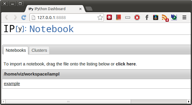
Click on example to open the notebook.

The notebook starts with an AMPL code for a simple transportation problem by George Dantzig. The first line of the cell is %%ampl which is a so called "cell magic" specifying that the rest of the cell contains AMPL code. You can execute the code by selecting the cell and pressing Shift-Enter. The AMPL interpreter stays running in the background so you can access the solution, modify the data and do other tasks as in the ampl console. There is a reset command at the beginning of the AMPL code which is not strictly necessary, but it is useful in case you want to re-run the cell for some reason. This avoids redefinition of AMPL objects such as sets and parameters.

In [1]:

%%ampl
reset;

set Plants;
set Markets;

# Capacity of plant p in cases
param Capacity{p in Plants};

# Demand at market m in cases
param Demand{m in Markets};

# Distance in thousands of miles
param Distance{Plants, Markets};

# Freight in dollars per case per thousand miles
param Freight;

# Transport cost in thousands of dollars per case
param TransportCost{p in Plants, m in Markets} :=
    Freight * Distance[p, m] / 1000; 

# Shipment quantities in cases
var shipment{Plants, Markets} >= 0;

# Total transportation costs in thousands of dollars
minimize cost:
    sum{p in Plants, m in Markets} TransportCost[p, m] * shipment[p, m];

# Observe supply limit at plant p
s.t. supply{p in Plants}: sum{m in Markets} shipment[p, m] <= Capacity[p];

# Satisfy demand at market m
s.t. demand{m in Markets}: sum{p in Plants} shipment[p, m] >= Demand[m];

data;

set Plants := seattle san-diego;
set Markets := new-york chicago topeka;

param Capacity :=
    seattle   350
    san-diego 600;

param Demand :=
    new-york 325
    chicago  300
    topeka   275;

param Distance : new-york chicago topeka :=
    seattle        2.5      1.7     1.8
    san-diego      2.5      1.8     1.4;

param Freight := 90;

solve;

MINOS 5.51: optimal solution found.
4 iterations, objective 153.675

You can mix AMPL code, text, markdown, Python code and even formulas written in LaTeX, for example: $$F(k) = \int _{-\infty}^{\infty} f(x) e^{2\pi i k} dx$$

At the end of the AMPL code there is a solve command so running the cell will also invoke the solver. You can, of course, split the AMPL code between several cells, for example, separating model and data. After running the AMPL code cell all the sets, parameters, variables, objectives and constraints become available in the IPython notebook and you can use them as normal Python objects.

For example, you can print values of objective and variables:

In [2]:

print 'Cost =', cost

# Indexed AMPL parameters, variables, constraints, etc. act as
# Python dictionaries.
print 'Shipment:'
for s in shipment:
    print s, shipment[s]

Cost = 153.675
Shipment:
('san-diego', 'topeka') 275.0
('seattle', 'topeka') 0.0
('san-diego', 'new-york') 275.0
('seattle', 'new-york') 50.0
('san-diego', 'chicago') 0.0
('seattle', 'chicago') 300.0

The value of an AMPL object can be accessed using the val property, for example cost.val. If the object is indexed over one or more sets, the value will be a dictionary.

And you can use matplotlib to visualize the data:

In [3]:

# It is easy to visualize the data using matplotlib.
s = shipment.val
pos = arange(len(s))
barh(pos, s.values(), align='center')
yticks(pos, s.keys())
show()

Web-based notebook is not the only interface to IPython. There is also a nice QT console and a terminal interface. To learn more about IPython go to its website where you can find plenty of learning material. I also recommend watching this nice talk by Fernando Perez "Science And Python: retrospective of a (mostly) successful decade":

Both IPython and iampl are open-source projects. IAmpl is still work in progress, so if you'd like to contribute or report a bug go to this GitHub repository.

Last modified on 2013-01-08